A Small Dice Game for the Kingman Formula

In a previous post I wrote about the relation between utilization, fluctuation, and waiting time, and its approximation by the Kingman formula. Let me show you a quick and easy dice game where we simulate a supermarket checkout to let participants experience the effect of utilization, fluctuation, and the (worse) combined effect of both.

Introduction

Waiting time in front of a process is heavily influenced by two things: the utilization of a process (how busy is it?) and the fluctuations of the arrival and process times (how steady is the system – or not?). The Kingman equation and others show this nicely (check out my post The Kingman Formula – Variation, Utilization, and Lead Time for details on the equation).  As the utilization approaches 100%, the waiting time approaches infinity. As the fluctuations of the arrival and process times increase, so does the waiting time. This game will demonstrate this effect.

\[ {  E(W) = \left ( \frac{p}{1-p} \right )\cdot \left ( \frac{ C_{a}^{2}+ C_{s}^{2} }{2} \right ) \cdot \mu_{s} } \]

Game Equipment

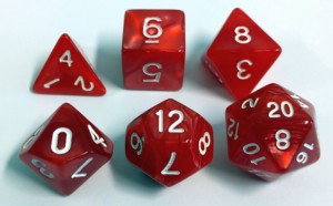
What you need are dice! Many-different-sided dice! If you grew up before the internet like me, then you may be familiar with dice that are different from the common six-sided dice D6 (Dungeons and Dragons anyone?).  In particular, you need three different types of dice – a small one (D4 or D6), a medium-sized one (D10 or D12), and a large one (D20 or D30).

Ideally you have one of each die for every player, but if you are short on dice you can have one die for every two players (we will make teams of two people shortly). It is best to have a large spread in the range of dice (i.e., using D4 as the smallest one and D30 as the largest one).

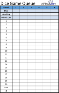Then you would need to print out the data sheets (one for every two players, plus maybe a few for backup). There is also an overview sheet, but you can also use a whiteboard, blackboard, or a flip chart for a quick sketch. More on  these below.

The game itself takes about one hour including some theory, and can handle a wide range of group sizes, although it does get cumbersome if you have more than thirty people.

The Game

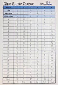
You will create groups of two people, each simulating a supermarket checkout. One will determine the number of people arriving, the other the capacity of the checkout. They get one dice-game queue-length sheet as shown above. Each then gets a die, which will determine the number of customers arriving at the checkout and the number of customers processed at the checkout. They may have to share one die if you are short on dice. There will be six rounds in the game, and each round consists of twenty iterations. In the first three rounds we vary the utilization.

Varying Utilization

Round 1 – D4 with Offset 2: In the first round, each player gets a four-sided die. For the number of people arriving, we throw the die and add 13. For the capacity of the checkout, we also throw a die, but this time add 15.  Therefore the checkout has on average two more capacity than the number of people arriving. This information would also be the first three empty rows on the data sheet, where we write 4 (for the sides of the die),  13 (for the customer), and 15 (for the supplier). This could also be printed on the sheet, but I prefer to keep the players in the dark on the future rounds so that they can focus on the current round.

Both throw the die and add to determine the arrivals and capacity. If the capacity matches or exceeds the demand, the two players write a zero in the next cell below. If the arrivals exceed the capacity, the number of people waiting is noted down. These people waiting in the queue have to be processed in the next iteration. They repeat this for twenty iterations, always keeping track of the number of people waiting in line. Afterward they calculate the total and average queue length by summing up the twenty entries and dividing by 20. This is written in the last two rows of the sheet.

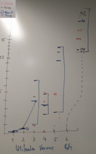
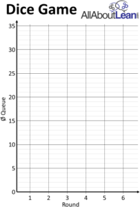The results are added to an overview statistic for all teams. A blank sheet is shown here, which could be printed or simply drawn on a whiteboard, blackboard, or flip chart. You write down the average queue length for each team in round 1. In all likelihood there will be no queue, as the expected outcome is 0.07 people waiting in line with a standard deviation of 0.08 people.

Round 2 – D4 with Offset 1: The next round we reduce the offset. The arrivals keep on adding 13 to the die, but the checkout now adds 14 (instead of 15) to his throw. Therefore the first three rows of round 2 are 4, 13, and 14. Again they play for twenty iterations and then determine the average queue length. These results will be added to the overview statistics for all teams.

The expected outcome is now an average queue of 0.5 people with a standard deviation of 0.4 people, so there will be more people waiting in line.

Round 3 – D4 with Offset 0: The next round we eliminate the difference between the arrivals and checkouts. Both can add only 13 to their die throw. Now the queue starts to heat up. The expected outcome is an average queue length of 3.1 people with a standard deviation of 2.3 people.

Theory on Utilization

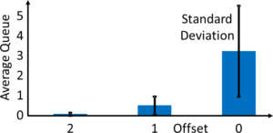At this point, we should discuss with the participants what happened. By reducing the overcapacity per iteration from 2 to 1 to 0, we in effect increased the utilization of the checkout. When the checkout had on average two more capacity than the people arriving, he had in effect a utilization of 88.57%. With an offset of 1, the utilization was 93.945%. Without any offset, the utilization was 100%. In the long run, an utilization of 100% means a queue length of infinity, but since we did only twenty iterations, we did not get that far. The graphs shows the expected average outcomes with the standard deviations for a D4 with different offsets.

Varying Fluctuation

In the next two rounds, we vary the fluctuations while keeping the offset constant. This means the utilization will always be at 88.57%.

Round 4 – D12 with Offset 2: Now we use a twelve-sided die. The arrivals add 9 to his throw, and the checkout adds 11 to his throw. Again, after twenty iterations, we add the averages to the overview sheet. The expected outcome is an average queue length of 3.0 people, with a standard deviation of 2.4.

Round 5 – D30 with Offset 2: Finally, we get to use the thirty-sided die. To maintain the same utilization and offset, the arrivals add nothing to his die throw, while the checkout adds 2 to every die throw.  The expected outcome is an average queue length of 14.7 people, with a standard deviation of 11.0.

Theory on Fluctuation

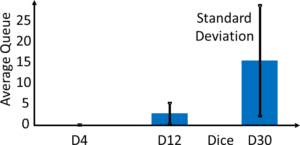By changing the die from a D4 to a D12 to a D30 while keeping the average arrivals and checkout capacity constant, we in effect increased the fluctuation. The D4 +13 arrivals meant that the number of arrivals fluctuated between 14 and 17 with an average of 15.5. A D12 +9 keeps the same average of 15.5, but now with a fluctuation from 10 to 21. A D30 plus nothing again has the same average of 15.5, but this fluctuates now between 1 and 30.

Hence, we increased the utilization. Similar to the utilization, increasing the fluctuation also increased the average backlog as shown in the chart above.

Varying Utilization And Fluctuation

Round 6 – D30 with Offset 0: For the next round we increase both fluctuation and utilization. Both the arrivals and the checkout get a thirty-sided die, and neither gets to add anything to the die throw. Important: Before we do this round, ask the participants about their guess on how long the queue will be! In all likelihood they will probably add the two effects together and expect a queue length of around 18. However, what they do not (yet) know is that these effects are not additive but more multiplicative! Let’s do the sixth round.

The expected queue length is not 18, but 24.2 people, with a standard deviation of 17.6. Hence it is much bigger than expected. Emphasize that this is not additive but multiplicative as per the Kingman equation above.

Simulation of Expected Outcomes

For your convenience, here is a table of the expected outcomes for offsets 2, 1, and 0 and for dice from two sides (a coin flip) to thirty sides in steps of two based on two hundred games each. Naturally, I did this in Excel rather than throwing a die eighteen thousand times . Besides, I don’t have a twenty-six-sided die, which according to Wikipedia wouldn’t really be a good die anyway. In any case, here is the mean and the standard deviation of the queue length for different situations.

	Mean Queue Length			Standard Deviation of Queue Length
Dice	Offset 2	Offset 1	Offset 0	Offset 2	Offset 1	Offset 0
2	0,00	0,00	1,21	0,00	0,00	0,88
4	0,07	0,49	3,07	0,08	0,42	2,28
6	0,47	1,35	4,80	0,39	1,11	3,59
8	1,01	2,89	5,80	0,79	2,99	4,03
10	1,88	3,86	7,70	1,50	3,35	5,48
12	2,98	5,39	10,26	2,44	4,45	7,25
14	3,91	6,83	11,71	3,33	5,75	7,90
16	5,49	7,33	13,24	4,88	5,32	8,60
18	6,04	9,56	14,62	4,93	7,42	10,35
20	8,22	11,99	15,67	6,95	9,26	11,83
22	9,85	12,33	19,17	8,23	9,19	13,67
24	10,92	14,19	20,51	9,39	10,56	14,30
26	12,44	16,99	23,02	10,92	11,70	16,17
28	11,89	18,65	22,83	9,13	13,44	15,75
30	14,70	20,36	24,18	11,02	14,49	17,64

Different Dice

If you don’t have a thirty-sided die, you can also use a twenty-sided die. If your largest die has only twelve sides, then it may be difficult to see a good effect. The numbers added to the arrivals for different dice above would work for any die up to 30, but if you have smaller dice, you can also use smaller add-ons. The table below shows you the quantity to add to the arrivals for different dice depending on your largest die. The numbers in any row would also work for any smaller dice. The checkout has to add 2, 1, or 0 on top depending on your desired utilization.

Dice	D4	D6	D8	D10	D12	D20	D30
Max D30	13	12	11	10	9	5	0
Max D20	8	7	6	5	4	0
Max D12	4	3	2	1	0

So, there it is, a quick and easy game with which you can demonstrate the effect on the backlog or waiting time of utilization and fluctuation, and the much-worse combined effect of utilization and fluctuation! I believe everybody can share that feeling if they are waiting at the supermarket checkout.

This game was inspired by the dice game in The Lean Games and Simulations Book by John Bicheno, which uses D6 to show the effect of utilization. I expanded this using different dice to also show the effect of fluctuation and the even-worse combined effect. Now, go out, throw a dice (not at your coworker, boss, or customer!), reduce fluctuation, get utilization under control, and organize your industry!

PS: Since publication of this post I also wrote an academic paper on this game: Roser, Christoph, and Masaru Nakano. 2018. “A Small Dice Game for the Kingman Formula.” In Proceedings of the International Conference on the Advances in Production Management System. Seoul, Korea.